Accelerating Swarms

The prospect of a Cambrian explosion of swarm intelligence has captured the zeitgeist (see: the Hugging Face hack), yet eliciting qualitatively new collective capabilities by scaling agent populations remains elusive. We posit such an explosion is unnecessary for vastly accelerating collective self-improvement, and improvements in how agents are organized and how knowledge is represented, validated, and accumulated can themselves alter the scaling of collective progress. Specifically, we argue the following:

• the progress of a swarm of $N$ agents can be modeled as a scaling curve in population size, time, and accumulated knowledge; time to a given performance target scales locally as $N^{-\lambda}$, so even small increases in the exponent can accelerate collective self-improvement by orders of magnitude;

• the exponent and the effective work per unit of compute depend on agent organization, structural task decomposition, and the methods used to represent, validate, and transfer knowledge;

• reusing intermediate results across agents and attempts increases effective work per unit of compute when avoided work exceeds validation, transfer, and maintenance costs; when this proportional improvement increases with population size, reuse also raises the exponent;

• together, these mechanisms allow accumulated knowledge to expand swarm capabilities while reducing the computation required for further learning, accelerating successive cycles of collective self-improvement.

To this end, we develop a probabilistic framework for forecasting and diagnosing collective improvement, and use it to identify high-expectancy research directions in agent organization, knowledge transfer, and verification.

1 The scaling curve

How much sooner can a larger swarm achieve a given level of performance? In Swarm Scaling, Ord addresses this question by approximating the performance of $N$ agents operating for time $t$ by that of a single agent operating for time $tN^\lambda$ [1]. Here, we can think of $\lambda$ as measuring how effectively computation parallelizes across the population; naturally, duplicated reasoning, sequential dependencies, and communication costs keep $\lambda$ generally below one.

Across three benchmarks, Ord estimates $\lambda$ between $0.48$ and $0.68$ [1, 2]. At sixteen agents, these estimates imply $3.8$–$6.6$ times the speed at $2.4$–$4.2$ times the total computation (Table 2). This suggests a trade-off between completion time and total computation. Raising $\lambda$ improves both, with speedup scaling as $s=N^\lambda$ and total-computation multiplier as $k=N/s=N^{1-\lambda}$.

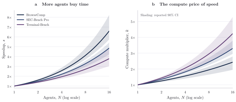
Ord’s relation compares the time and computation required to reach the same performance at different population sizes. We extend this description to account for differences in task difficulty and for accumulated knowledge that makes subsequent tasks easier to solve. To measure progress consistently, we consider a fixed set of tasks with explicit criteria for successful completion.

Let $r_j$ denote the baseline completion rate of task $j$ for a single agent that uses fixed methods and initial knowledge. Organization and accumulated knowledge affect how efficiently tasks are solved, so as a first approximation, we represent their effect by a common multiplier $A(t,N)$, determined by the retained useful knowledge $H(t)$ and the population size $N$. Incorporating Ord’s population scaling gives the completion rate conditional on task $j$ remaining unsolved, $$h_j(t,N):=r_jN^\lambda A(t,N).$$ The probability that task $j$ remains unsolved after time $t$ is then $$\Pr(T_j>t) =\exp\!\left[-\int_0^t h_j(u,N)\,du\right] =\exp[-r_jW(N,t)],$$ where $T_j$ is completion time and $W(N,t):=N^\lambda\int_0^t A(u,N)\,du$ is cumulative effective computation. This separates the computation supplied by the swarm, $W(N,t)$, from the difficulty of each task, represented by $r_j$.

We want $r_j$ to capture variation in task difficulty, which is substantial even among tasks requiring comparable human effort. Among accessible tasks, a natural model is $$r_j\sim\operatorname{Gamma}(a,\mathrm{rate}\ b),$$ since the Gamma distribution allows arbitrarily low completion rates and yields an explicit expression for average failure. At fixed $b$, smaller $a$ places more probability on tasks with low completion rates; at fixed $a$, increasing $b$ proportionally increases the effective computation required for the same performance.

We let $Q(N,t)$ denote the expected fraction of tasks remaining unsolved, and let $q$ be the fraction inaccessible throughout the modeled regime, i.e. with completion rate zero. Averaging over the remaining tasks using the Laplace transform of the Gamma distribution gives $$\begin{equation} \boxed{ \begin{aligned} Q(N,t) &\approx q+(1-q)\,\mathbb E_{r_j}\!\left[e^{-r_jW(N,t)}\right] \\ &=q+(1-q)\left[1+\frac{W(N,t)}{b}\right]^{-a}. \end{aligned} } \end{equation}$$(1) The curve describes how additional effective computation reduces failure toward the floor $q$. Inverting this gives the effective computation required to reach a target $Q^\star>q$, $$\begin{equation} \boxed{ W(N,t^\star)\approx b\left[\left(\frac{1-q}{Q^\star-q}\right)^{1/a}-1\right]. } \end{equation}$$(2) When the efficiency factor $A$ is constant over the evaluation interval we have $W(N,t)=tN^\lambda A$, so the time to target is given by $$\begin{equation} t^\star = \frac {W(N,t^\star)}{N^\lambda A} \approx \frac b{N^\lambda A} \left[\left(\frac{1-q}{Q^\star-q}\right)^{1/a}-1\right]. \end{equation}$$ Total computation is then $Nt^\star$, assuming equal, constant computational rates per agent.

The scaling curve provides a common framework for comparing changes in organization and accumulated knowledge at matched performance. For a fixed task distribution, faster progress requires more agents $N$, greater per-agent efficiency $A$, or a higher effective scaling exponent $\lambda$. This makes duplicated work, sequential dependencies, and communication overhead concrete constraints for better organization to address.

2 Organization and knowledge representation

2.1 Organization as a distributed decision problem

The scaling curve in Equation 1 summarizes the effects of organization through the efficiency factor $A$ and the population-scaling exponent $\lambda$. This gives us a way to investigate how a swarm should allocate computation to acquire and use knowledge so as to reduce the time and computation required for further progress.

A difficulty is that estimating a computation’s expected contribution to collective progress requires information distributed across the population. An experiment with little immediate value to the agent conducting it may resolve uncertainty shared by many other agents’ attempts. Conversely, a promising experiment may duplicate work elsewhere. Choosing what to compute therefore requires estimates of both the dependencies between outstanding problems and the knowledge already available to resolve them.

Acquiring such distributed information consumes resources. For example, determining whether another agent has resolved a subproblem may require searching its records and reconstructing its reasoning, while estimating which agent is best suited to an experiment may require preliminary evaluations. Organization thus involves jointly deciding what to investigate, what to communicate, and how to allocate work conditional on the resulting evidence.

The potential savings grow when many attempts share dependencies that would otherwise be resolved separately (as we expect increasingly in larger swarms). Realizing these savings requires representations through which agents can identify and reason about those dependencies.

2.2 Knowledge primitives

A knowledge primitive specifies a representation of knowledge together with operations for querying, updating, and combining its contents. For example, suppose a swarm is evaluating candidate algorithms under a limited experimental budget. A knowledge primitive could then represent a joint probability distribution over their performance. With efficient primitives, conditioning on an experimental result updates predictions for many statistically dependent algorithms; then observations from multiple agents are easily combined by conditioning on their pooled evidence.

We therefore ask, which dependencies can the swarm learn and exploit cheaply enough that evaluating one candidate reduces the computation needed to assess others?

Pooling evidence requires deciding how much information each agent should transmit and how recipients should incorporate it. Tanaka illustrates the consequences in a naming game, where agents repeatedly choose a label for a shared referent [3].

In this game, each agent maintains a probability distribution over possible labels, samples a label to communicate, and increases the probability of labels it receives from others. A label selected by chance therefore becomes more likely to be transmitted again. Through successive exchanges, this reinforcement can produce population-wide agreement even when agents initially assign equal probability to every label and receive no external evidence favoring one.

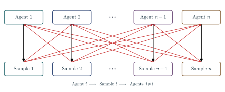
Communicating more samples reduces this reinforcement by conveying the sender’s distribution more accurately. Tanaka shows that sampling contributes an expected increase in collective agreement per interaction proportional to $1/s$, where $s$ is the number of independent samples per message, and observes approximately this dependence in GPT-4o naming-game experiments.

Both examples suggest that the effectiveness of allocation depends on how knowledge primitives represent dependencies and update agents’ beliefs as information is exchanged.

2.3 Task decomposition and agent allocation

Knowledge primitives provide a basis for deciding how to decompose tasks and allocate agents. By representing unresolved subproblems and their dependencies, they help agents estimate which investigations can proceed in parallel, where additional agents would accelerate completion, and when to revise the approach. The total work and sequential depth of a proposed decomposition quantify the constraints on this allocation, allowing us to examine how decomposition affects population scaling.

For a task $j$, agent $i$ uses its retained knowledge $H_i$ to select an approach $a$ and decomposition $d$. We represent this selection by a proposal policy $\pi_{\theta_i}$, $$(a,d)\sim\pi_{\theta_i}(\,\cdot\mid j,H_i),$$ whose parameters $\theta_i$ encode the agent’s research taste through its preferences over hypotheses, methods, and decompositions.

Allocating agents to a proposal then requires estimating both how much computation it entails and how much can proceed in parallel. These requirements are uncertain given the agent’s current knowledge, so we represent its estimates by a predictive distribution $p_i$, $$(B,D)\sim p_i(\,\cdot\mid a,d,j,H_i),$$ where the total remaining work $B$ is the total computation required to complete the subtasks, and the sequential depth $D$ is the sum of subtask durations along the longest dependency path, both measured in single-agent computation units.

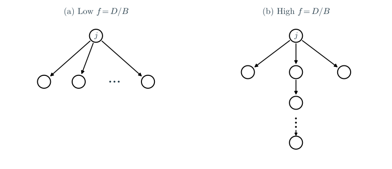
These estimates constrain how much a proposed decomposition can benefit from additional agents. Conditional on work $B$ and depth $D$, a team of $m$ equally fast agents requires at least $$T_m\geq\max\left(\frac{B}{m},D\right)$$ to complete the fixed dependency graph, since distributing the work perfectly would take $B/m$, while the longest dependency path requires time $D$. Ignoring additional communication and scheduling overhead, Brent’s theorem gives an execution time of $\Theta(B/m+D)$ [4]. The ratio $B/D$ therefore indicates how many agents the decomposition can use effectively; once $m$ exceeds this scale, completion time is increasingly constrained by longest dependency path.

Consider a decomposition with a serial component requiring computation $D$ and a perfectly divisible parallel component $B-D$. Ignoring coordination overhead, its completion time is $$T_m=D+\frac{B-D}{m}.$$ Writing $f=D/B$, its speedup and local population-scaling exponent are then $$s(m)=\frac{B}{T_m} =\frac{m}{1+f(m-1)}, \qquad \lambda_{\mathrm{team}}(m) =\frac{d\log s(m)}{d\log m} =\frac{1-f}{1+f(m-1)}.$$

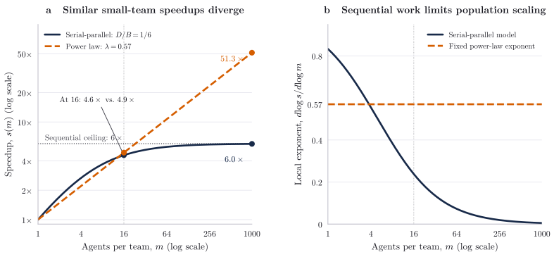
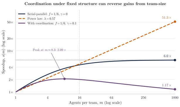
From here, we can see that for a fixed decomposition, adding agents eventually leaves completion time dominated by sequential work. At $m=B/D=1/f$, the local exponent is $(1-f)/(2-f)$, approximately $1/2$ when $f$ is small and it approaches zero as team size grows further. Figure 5 illustrates why this matters for extrapolation: at sixteen agents, the serial–parallel model with $D/B=1/6$ and the power law with $\lambda=0.57$ both give roughly fivefold speedup. At a thousand agents, their predictions diverge to approximately sixfold and fifty-onefold. Similar performance at small populations can therefore conceal substantially different limits to scaling.

The ratio of sequential depth to total work is a core bottleneck. Similarly, sustaining the rate of improvement with population size requires organization to expose additional parallel work. For example, a team can revise its decomposition to shorten a dependency chain, or use a retained result to eliminate a blocking subtask. Allocation therefore requires estimating both the work an agent could complete under the current decomposition and how its knowledge or methods could reduce the remaining work $B$ or sequential depth $D$.

These estimates depend on information held by teams and prospective contributors. The team knows which dependencies currently constrain its progress, while agent $i$ may possess methods or results in $H_i$ that could resolve them. Knowledge primitives can make these dependencies and potential contributions explicit, allowing each side to assess a proposed allocation using the information available to it.

One candidate policy is mutual acceptance. The agent considering joining an existing team proposes an investigation with a target subtask, computational budget, and expected output; the team assesses how that output would affect its remaining work and completion time. The agent compares the proposal with alternative uses of its computation, either independently or with other teams, while the team compares it with alternative ways of advancing its approach. If both select the proposal, the agent joins for the agreed investigation, with its allocation reconsidered as new evidence becomes available.

The effectiveness of this policy depends on how well pairwise estimates of investigation value capture swarmwide impact, as e.g. simultaneous proposals may duplicate work, an investigation may benefit several teams, or contributions are useful only in undiscovered combinations. This makes learning representations and allocation policies jointly all the more important, since representations determine which consequences agents can anticipate and policies determine how those estimates guide decomposition and allocation.

2.4 Learning how to organize computation

Sutton’s Bitter Lesson argues for general methods that scale with computation (particularly search and learning) over approaches built around hand-engineered domain knowledge [5]. The lesson motivates a meta-method that uses computation to improve how agents represent dependencies, propose decompositions, estimate their computational requirements, and locally allocate themselves to the resulting work.

We can evaluate the resulting organization by comparing the times $t_0^\star$ and $t_1^\star$ required to reach a common performance target before and after learning respectively. Over intervals where each organization’s efficiency is approximately constant, we have $W_i(N,t)\approx tA_iN^{\lambda_i}$, giving $$\frac{t_0^\star}{t_1^\star} \approx \frac{A_1}{A_0}N^{\lambda_1-\lambda_0},$$ i.e. the speedup from learning organization.

A learned policy may require more coordination per agent while using additional agents more effectively, lowering $A$ but raising $\lambda$. Its advantage then depends on population size. For example, if $A_1/A_0=0.8$ and $\lambda_1-\lambda_0=0.1$, the learned policy is approximately $6\%$ faster at sixteen agents and $60\%$ faster at a thousand. Search conducted only on small populations could therefore discard policies that would substantially accelerate larger swarms.

To determine whether these improvements reduce total computation, we must include the cost of learning the policy. If learning consumes $C_{\mathrm{learn}}$, and task instance $j$ requires computation $C_{0,j}$ under the initial policy and $C_{1,j}$ under the learned policy at matched performance, the investment is recovered when $$\sum_{j=1}^{J}(C_{0,j}-C_{1,j})>C_{\mathrm{learn}}.$$ Because the learning cost is incurred once while savings accumulate across subsequent uses, methods that generalize broadly can justify a larger initial investment in learning organization. Thus, learning how to organize computation can itself accelerate collective self-improvement, as the resulting methods reduce the computational cost of subsequent discoveries.

3 Reuse, verification, and transfer

3.1 Preserving intermediate progress

The same principle of recovering computational investment through reuse applies to intermediate results within a task. The idea is that if a completed subproblem can be verified independently, subsequent attempts need only succeed on the unresolved subproblems. For tasks with successive stages, this can change the expected computation required for completion from exponential to linear in task depth.

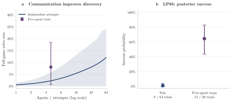
Experiments with communicating agents suggest that sharing intermediate results can reduce the computation required to solve tasks. Across 25 ARC-AGI-3 games, five communicating agents achieved an 8.0% full-game solve rate, compared with 2.2% for the best of five independent attempts. Moreover, increasing the number of independent attempts to match the team’s solve rate required approximately 4.9 times the team’s output-token expenditure [6].

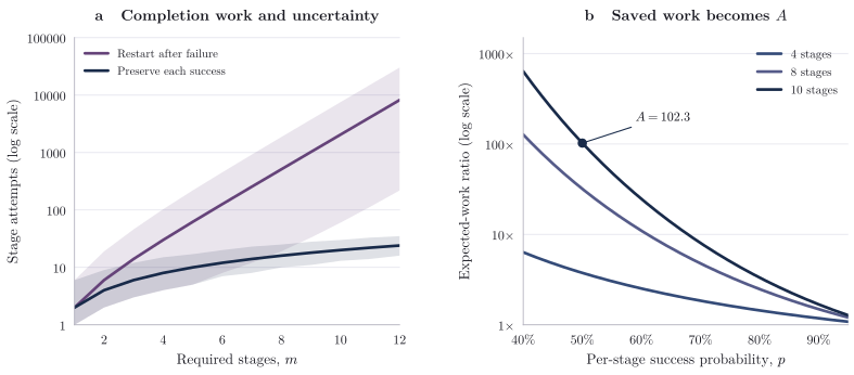
To quantify the effect of preserving intermediate progress on expected computational cost, we consider a task requiring $m$ successive stages, each completed with probability $p$ per independent, unit-cost attempt. Suppose completed work is preserved every $\ell$ stages, so failure requires only the current block to restart. Assuming $\ell$ divides $m$, checkpoints are valid, and verification, retrieval, and storage costs are negligible, expected computation is $$C_\ell = \frac{m}{\ell}\frac{1-p^\ell}{(1-p)p^\ell}.$$ For fixed $0<p<1$, keeping checkpoint spacing fixed therefore makes expected computation grow linearly with task depth, whereas restarting produces exponential growth. At $m=10$ and $p=0.5$, expected computation falls from 2,046 stage attempts with no intermediate checkpoints to 30 when preserving every two stages, and 20 when preserving every stage.

This calculation assumes that valid checkpoints are available every $\ell$ stages. In a swarm, the achievable spacing depends on whether the chosen knowledge primitive exposes intermediate results that can be verified and reused independently. Designing representations that support finer checkpoints could therefore reduce repeated computation, provided the savings exceed the additional verification and retrieval costs.

For example, suppose agents use the same Bayesian linear regression model to analyze separate batches of observations. Rather than retaining only fitted coefficients, each agent could save $X^\top X$ and $X^\top y$, where $X$ contains its batch’s predictors and $y$ its observed responses. For a shared prior and fixed noise variance, summing these quantities across disjoint batches gives the same posterior over coefficients as processing the pooled data. Each processed batch therefore provides a reusable checkpoint, allowing later agents to extend the analysis without repeating the earlier data processing.

3.2 Verification and controlling error propagation

The checkpoint model above assumes that verification accepts only valid intermediate results. We now relax this assumption and trace the consequences of a false acceptance to determine for what levels of reuse and verification reliability the expected number of downstream errors remains bounded.

To quantify this propagation, suppose each accepted result is used in $\kappa$ subsequent computations. If the result is incorrect, let $u$ be the probability that a downstream computation produces an incorrect result that also passes verification. We approximate the dependencies by a tree, so each downstream result has one parent, and hold $\kappa$ and $u$ constant across generations.

Let $Z_d$ count the incorrect, accepted results at depth $d$, starting with $Z_0=1$. Each produces $\kappa u$ further accepted errors in expectation, giving $\mathbb E[Z_d]=(\kappa u)^d.$ The expected total through depth $D$, including the initial error, is therefore $$\mathbb E[F_D] =\sum_{d=0}^{D}(\kappa u)^d = \begin{cases} \dfrac{1-(\kappa u)^{D+1}}{1-\kappa u}, & \kappa u\neq1,\\[6pt] D+1, & \kappa u=1. \end{cases}$$ For $\kappa u<1$, this expectation approaches $1/(1-\kappa u)$ as depth increases. At $\kappa u=1$, it grows linearly with depth; for $\kappa u>1$, it grows exponentially.

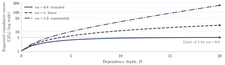
We can extend this model to include new false acceptances in each round of computation. Let $x_d$ denote the expected number of accepted errors generated in round $d$, and suppose each round introduces an expected $\eta$ new errors that do not descend from those already propagating. If each accepted error produces its downstream results in the next round, the same branching approximation gives $$x_{d+1}=\kappa u\,x_d+\eta, \qquad \lim_{d\to\infty}x_d=\frac{\eta}{1-\kappa u} \quad\text{when }\kappa u<1,$$ where we can interpret the factor $1/(1-\kappa u)$ as measuring how propagation amplifies the ongoing introduction of errors. Verification therefore affects the limiting error count through both the rate of new false acceptances, $\eta$, and the probability of propagating an accepted error, $u$.

These calculations treat $u$ and $\eta$ as fixed, but both depend on the proposals submitted to verification. When agents revise proposals using earlier evaluation feedback, they can select for apparent improvements specific to the evaluation data. A false-acceptance guarantee for a proposal chosen independently of that data therefore need not hold for proposals generated through this process. Reusable-holdout methods address this dependence by restricting the feedback released to the search procedure [7].

For example, Thresholdout compares a candidate’s performance on training and holdout data using a randomized discrepancy threshold. When the estimates agree sufficiently, it returns the training estimate; otherwise, it returns a noise-perturbed holdout estimate and reduces a finite disclosure budget. Once that budget is exhausted, it stops answering queries. This limits the information available for fitting subsequent candidates to the holdout data while retaining guarantees on evaluation accuracy [7].

Organizational policies must determine what evaluation feedback agents receive and share, while preserving accuracy guarantees across the swarm’s combined adaptive search.

3.3 Efficient verification

Controlling error propagation requires reliable verification, but this consumes computation. When an agent proposes a method for other agents to adopt, one form of verification is to establish whether it improves performance over their current method. We want to reduce the cost of this comparison while maintaining its reliability.

Evaluating both methods on the same tasks helps distinguish improvements from differences in task difficulty. Coordinating sample randomness can further reduce uncertainty. For example, coupled token generation uses the same underlying random numbers to sample tokens from different language models. In benchmark evaluations of Llama, Mistral, and Qwen models, it required up to $75\%$ fewer samples to reach the same benchmark conclusions as independent sampling [8]. Similar coordination could reduce the computation a swarm spends evaluating proposed improvements.

Further savings are possible when one evaluation informs several comparisons. For example, suppose agents are comparing algorithms that combine different search procedures and stopping rules. Under a simple additive model, algorithm $j$ has expected performance $a_j^\top\theta$, where $a_j$ records its components and $\theta$ their unknown contributions. Evaluating one algorithm provides evidence about those contributions, informing estimates for other algorithms that share its components. Best-arm identification in linear bandits uses this shared structure to choose which algorithms to evaluate, and how often, to identify the best at a specified confidence [9]. This provides a way for agents to allocate verification work according to the comparisons each evaluation helps resolve.

Reusing evaluation results across comparisons requires knowledge primitives that record which methods share components and the evidence available about their contributions to performance.

3.4 The computational value of reuse

To determine how much computation reuse saves, we must account for the cost of verifying and sharing results. Suppose $N$ agents each need a calculation costing $S$, followed by work specific to their task costing $P$. Working separately costs $N(S+P)$. Computing the shared result once reduces this to $S+NP+O(N)$, where $O(N)$ includes verification, retrieval, transfer, and maintenance. At matched performance and reliability, the work-efficiency multiplier is $$A_{\mathrm{reuse}}(N) =\frac{N(S+P)}{S+NP+O(N)}.$$ Reuse therefore saves computation when $O(N)<(N-1)S$.

As the population grows, the initial calculation is shared across more agents, but each use may still require retrieval, verification, and adaptation. Suppose these recurring costs are $c$ per agent, giving $O(N)=cN$. Dividing total computation by $N$ gives a cost per agent of $S/N+P+c$. When $c<S$, reuse saves computation at sufficiently large populations, but its efficiency multiplier eventually approaches $(S+P)/(P+c)$ for $P+c>0$.

When the proportional savings from reuse increase with $N$, reuse also raises the population-scaling exponent $\lambda$. When $A_{\mathrm{reuse}}(N)$ multiplies effective computation with the other scaling factors held fixed, its contribution to the local exponent is $$\Delta\lambda(N) =\frac{d\log A_{\mathrm{reuse}}(N)}{d\log N}.$$ With recurring costs $O(N)=cN$, the contribution to the exponent approaches zero as the savings saturate. Reusing the same result across more agents continues to save computation, but sustaining an exponent gain requires finding additional opportunities for reuse as the population grows. This motivates representations that help agents identify shared subproblems, provided the cost of verifying and transferring results remains below the computation avoided.

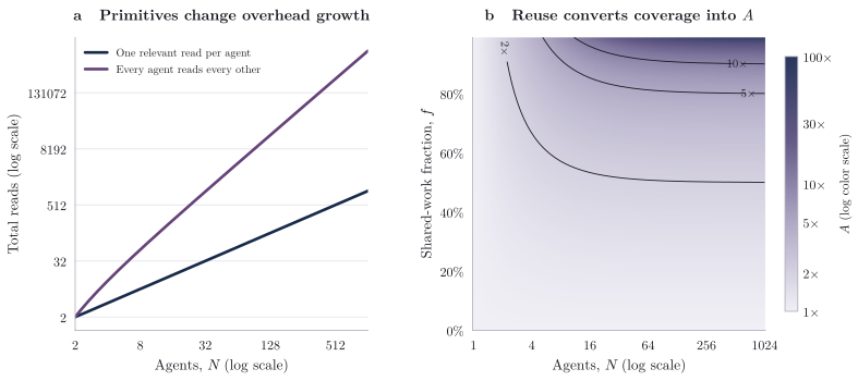
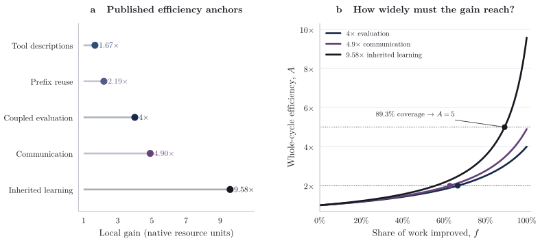
The overall saving also depends on how much of the workflow improves. If a method reduces the computation required for a fraction $f$ of the workflow by a factor $r$, then $$A_{\mathrm{workflow}}=\frac{1}{(1-f)+f/r}.$$ For example, if verification accounts for two-thirds of the original computation, making it four times cheaper at matched reliability halves the total computation required. Appendix A.5 gives the empirical efficiency estimates and coverage assumptions used in our forecasts.

This suggests learning which results to preserve and share according to the computation they are expected to save across the swarm, after accounting for verification and transfer costs.

3.5 Selective transfer and exploration

Sharing an improved method can reduce repeated work, but it may also lead agents to abandon alternatives before enough evidence is available to assess them. We want to determine when further evaluation of those alternatives justifies its computational cost.

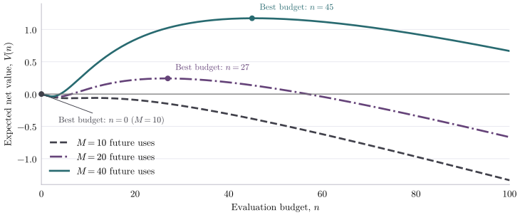
Suppose the current method has known expected performance $\mu_0$, and the swarm’s belief about an alternative’s expected performance is $\mu\sim\mathcal{N}(m,\tau^2)$, with $\Delta=\mu_0-m>0$. Each evaluation returns $Y_k=\mu+\epsilon_k$, where the errors are independent $\mathcal{N}(0,\sigma^2)$. Furthermore, suppose the swarm evaluates the alternative $n$ times, then chooses a method for $M$ subsequent uses. Specifically, it adopts the alternative if its updated expected performance $m_n$ exceeds $\mu_0$; otherwise, it retains the current method. Before observing the evaluation results, $$m_n\sim\mathcal{N}(m,s_n^2), \qquad s_n^2=\frac{\tau^4}{\tau^2+\sigma^2/n}.$$ Relative to using the current method throughout, the expected gain over $M$ subsequent uses, after subtracting the evaluation cost $cn$, is then $$\begin{aligned} V(n) &=M\,\mathbb{E}\!\left[(m_n-\mu_0)_+\right]-cn\\ &=M\left[s_n\phi\!\left(\frac{\Delta}{s_n}\right) -\Delta\Phi\!\left(-\frac{\Delta}{s_n}\right)\right]-cn, \end{aligned}$$ where $\phi$ and $\Phi$ are the standard normal density and distribution functions, $(x)_+=\max(x,0)$, and $c$ includes evaluation and opportunity costs in the same units as total performance.

When $s_n$ is small relative to the performance gap $\Delta$, the evidence is unlikely to change the swarm’s choice of method. A larger budget can make that evidence sufficiently informative to justify switching, with the expected benefit increasing in the number of subsequent uses $M$. However, this benefit is bounded as $s_n$ approaches $\tau$, while evaluation costs grow linearly with $n$. The allocation rule under this model is therefore to choose the budget that maximizes $V(n)$, including $n=0$ as the option of retaining the current method without further evaluation. Figure 10 shows how the best choice can be an intermediate budget even when a single evaluation has negative net value.

The next question is how to allocate a shared evaluation budget across several alternatives. As in Section 3.3, evidence about shared components can inform several candidates, so the value of investigating one alternative depends on what other investigations will reveal. Cheaper verification can also make previously unprofitable investigations worthwhile. This suggests learning allocation policies that account for these dependencies and revise investigation budgets as evidence accumulates.

4 Accumulation and accelerating improvement

4.1 Feedback

There are already some narrow instances of automated work feeding back into AI development. AlphaEvolve reports a 23% average kernel speedup from an evolved heuristic, corresponding to a 1% reduction in overall Gemini training time [10]. Automated search has also extended to multiagent learning algorithms [11].

To specify, as $H(t)$ accumulates, discoveries can reduce future work, where e.g. discovering a new simulator or retaining a method can reduce operational cost, so $A(t, N)$ rises. Note that, dependent on the policy of researchers, we can tune the proportion of work that is estimated to be useful in the future. If encouraged to optimize for research throughput, the agent may (dependent on horizon) favor reusable discoveries that accelerate subsequent investigations.

Lower experimental cost can notably: 1) allow the same experiments to run faster, lowering $\tau_k$, the duration of a given research cycle; and 2) allow more experiments to run in parallel within a given compute constraint. Particularly, this can make experiments with large upfront costs worthwhile when their results are useful at scale.

To formalize this, let $G_k$ be the retained log improvement in cost-adjusted research productivity after cycle $k$. At a fixed population and quality target, it is the reduction in log completion time from our common curve, $$G_k=-\Delta\log t.$$ Holding the task distribution fixed, this reduces to $\Delta\log A+\Delta\lambda\log N$. If successive research cycles require the same effective work, this gives $\tau_{k+1}=\tau_k e^{-G_k}$. More generally, let $w_k$ denote the effective work required for cycle $k$, measured in the same baseline units across cycles. Then $$\frac{\tau_{k+1}}{\tau_k} =\frac{w_{k+1}}{w_k}e^{-G_k}.$$ Successive cycles become shorter when productivity gains outpace the growth in required work, $$G_k>\log\frac{w_{k+1}}{w_k}.$$

Now we consider our actual effective work over the duration of our experiments. Suppose each gain $G_k$ is deployed at time $t_k$ and remains available thereafter, with productivity unchanged between deployments. Since $G_k$ is a log productivity gain, each deployment multiplies the rate of effective work by $e^{G_k}$. At a fixed population $N$, this gives $$N^{\lambda(u)}A(u,N) =N^{\lambda(0)}A(0,N)\exp\left(\sum_{k:t_k\leq u}G_k\right).$$ Then for total effective work we have $$W(N,t)=\int_0^t N^{\lambda(u)}A(u,N)\,du=A(0,N)N^{\lambda(0)} \int_0^t\exp\left(\sum_{k:t_k\leq u}G_k\right)\,du.$$ As an example, suppose each cycle requires the same effective work and yields a gain $G_k=\log 2$ upon completion. Successive cycles then take $\tau_0$, $\tau_0/2$, and $\tau_0/4$, giving $$W(N,7\tau_0/4)=3N^{\lambda(0)}A(0,N)\tau_0,$$ i.e. three cycles’ effective work is completed in 1.75 initial cycles’ time!

To examine asymptotic behavior, we can let $G(t)$ smoothly approximate the cumulative log gain $\sum_{k:t_k\leq t}G_k$ when individual gains are small and many improvements occur over the timescale of interest. Then $$W(N,t)\approx N^{\lambda(0)}A(0,N)\int_0^t e^{G(u)}\,du,$$ giving $W'(N,t)\approx N^{\lambda(0)}A(0,N)e^{G(t)}$ and $W''(N,t)\approx G'(t)W'(N,t)$. Equivalently, $$\frac{d}{dt}\log W'(N,t)\approx G'(t),$$ i.e. the rate of accumulated log improvement determines the proportional growth rate of research throughput! It is reasonable to expect this speedup to shift the bottlenecks constraining subsequent research, making the trajectory difficult to predict in advance [12].

4.2 Addressing limitations

4.2.1 Context degradation and swarm knowledge

For a single agent, a longer investigation can make reliable use of context more difficult. As information accumulates, subsequent actions are conditioned on a history containing relevant evidence alongside noisy attempts that accompanied the discovery process. The core difficulty is in distinguishing what information should still guide subsequent work.

For swarms, the information retained from an investigation need not be the full context in which it was conducted. For instance, agents can use the verification mechanisms in Section 3 to preserve validated results separately from the attempts that produced them. Subsequent agents can then retrieve those results into fresh working contexts, building on earlier discoveries without also inheriting the irrelevant or superseded material. As a result, learning accumulates at the organizational level without requiring each agent to retain the organization’s entire history.

This requires agents to find and integrate relevant results as the repository grows. Section 3.4 considers a bounded number of reads per agent, giving $O(N)$ reads across the population. Sustaining this bound requires retrieval methods that locate useful results without making agents inspect progressively more records, which can be improved by reorganizing its accumulated knowledge. A-MEM provides an example of adaptive memory organization. Newly added memories are linked to related records and can trigger updates to the contextual descriptions and attributes of existing memories [21]. Self-organization extends to the knowledge agents leave for subsequent investigations, with improvements to its organization reducing retrieval costs across future uses.

4.2.2 Global approaches

The paper is structured around a swarm built on local agentic interactions. Why emphasize this design instead of directing the swarm through a central coordinator? We wanted to avoid using institutions and analogies from human organization to prescribe agents’ roles and interactions. While human organizational structures reported more coherent solutions on collaborative software-engineering benchmarks, irregular collaboration topologies could outperform regular ones  [19, 20]. Swarms do not need to be constrained by natural existing structures. Human organizational structures developed under constraints on memory, communication, and the transfer of expertise that need not apply in the same way to agents. Agents can be copied and forked from a shared state, while knowledge primitives can support querying and combining intermediate results without requiring human-readable explanations of each operation. These capabilities change which divisions of work and forms of communication are efficient. Following Sutton’s Bitter Lesson, we instead want to use search and learning to discover effective organization under the computational and communication constraints agents actually face [5].

Suppose we consider a natural reporting hierarchy as a balanced $x-$ary tree with $m$ worker agents at its leaves and $x\geq2$ reports per manager node, making the depth $\lceil\log_x m\rceil$. Suppose each manager processes its child reports serially at cost $c$ per report, and managers of the same level are parallelized. One upward reporting through the tree takes $$T_{\mathrm{coord}}\approx xc\lceil\log_x m\rceil,$$ subject to sufficient manager capacity. Including the runtime from work–depth decomposition, the total time to complete a task is then $$T_m\approx T_{\mathrm{work}}+xc\lceil\log_x m\rceil \implies T_{m}=\Theta\!\left(\frac{B}{m}+D + xc\lceil\log_x m \rceil \right),$$ from Section 2.3. Observe $x \log_x m = x \frac{\log m}{\log x},$ which is minimized when $x = e$ or $x = 3$ when restricted to integers. Let $\gamma = \frac{3c}{B \log 3}$ which represents the coordination cost per unit work. Doing the same analysis from Section 2.3 yields $T_m = D + \frac{B - D}{m} + \gamma B \log m$ and $$\lambda(m) = -\frac{d\log T_m}{d\log m} = \frac{1 - f - m \gamma}{1 + f(m - 1) + \gamma m \log m},$$ as the effective team-scaling exponent. While some coordination cost $\gamma > 0$ is present under any organizational structure, the $\gamma\log m$ term in $T_m$ arises from required reporting under the $x-$ary tree. Certainly imposing a structure can warm-start organization and increase efficiency in allocation for small $m$. But fixing the structure caps useful team size as $m$ grows, motivating local self-organization where agents can potentially learn to avoid aggregating information through middle managing hierarchies.

4.3 Why we are optimistic

There are many reasons to be excited here. One of the safest bets in technological development is on Moore’s Law; as compute rises, it is reasonable to expect that the bottleneck in deploying experiments will be in speed, pushing swarms to the forefront (as seen with e.g. Navier-Stokes). Consequently as swarms become a greater focus in inference time-compute scaling, more resources will be deployed towards improving the machinery of collaboration.

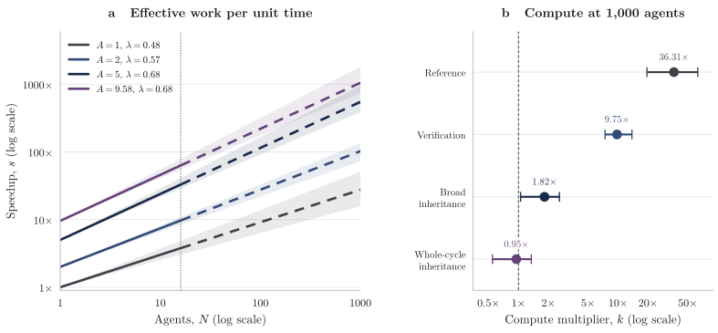
As a base rate, even severe diminishing returns leave room for extraordinary acceleration: taking $\lambda=0.5$, a thousandfold increase in concurrent research effort still compresses a month of discovery into a day. Swarming is incubatory, and populations much larger than those used to fit current curves are already being explored [14]. As more resources are allocated towards swarming, e.g. a rise in SoTA swarms from size $10^4 \to 10^6$ leads to a tenfold increase in research speed. Scaling laws lean heavily in favor of swarm organization accelerating recursive improvement drastically. As an example, see Table 3 and corresponding Figure 12.

The nascence of swarms suggests that there are many low-hanging fruits in improving domain-specific collaboration through smart selection of primitives, better verification, and efficient transfer established through e.g. smart harnesses and infrastructure. To this end, we observe a recursive loop where domain-specific taste provides strong feedback, estimates, and counterfactuals, improving priors and raising the quality of data for the consequent self-organization of the swarm to its respective domain. In this sense, domain knowledge can provide a better sandbox for swarm experiments, accelerating the research loop (and consequently raising not only its initial speed and compute efficiency, but also these qualities’ rate of improvement).

For intuition, say by domain-specific application we can raise $\lambda$ by 0.1 above the general baseline; then as swarms get larger by virtue of interest, say $10^4 \to 10^6$, our speedup goes from $10^{0.4} \to 10^{0.6}$, i.e. we actually go from 2.5x to 4x speedup, i.e. domain speedups become more valuable as more resources are allocated towards the generalist scaling problem!

Now, consider that these researchers plausibly improve the machinery running them.

Today’s agents exchanging messages are an early implementation of a much more efficient system of shared computation. We should assign substantial weight to a future where this feedback compresses research timelines by many orders of magnitude, even if agent-specific capacity grows only modestly per unit of time (and actually depreciates per unit of experiment time!).

A Appendix

A.1 Parallelization estimates

Ord reports $\lambda$ and 90% intervals from the published one-, four-, and sixteen-agent curves. The speed band is $[A N^{\lambda_L},A N^{\lambda_U}]$; the compute band is $[N^{1-\lambda_U}/A,N^{1-\lambda_L}/A]$. Figure 12 propagates these intervals to the forecast populations, conditional on fixed $A$ and continuation of the fitted scaling relation. Coverage $f$ is shown separately in Figure 13. The source studies report point estimates or maxima for the efficiency anchors.

A.2 Communication and heterogeneous difficulty

For $s_j$ successes in 64 solo trials, the observed-pool best-of-$N$ expectation is $1-\binom{64-s_j}{N}/\binom{64}{N}$. The reconstructed counts are 22 zeros, two ones, and one six. Five-agent counts are 13, 4, 20, and 3 successes on LP85, AR25, FT09, and SB26, with zero on the remaining 21 games and 20 trials per game. Figure 6(a) uses 20,000 bootstrap resamples of the 25 games, retaining each game’s trial pool. Its pointwise 95% intervals describe variation under sampling games from this empirical population. LP85 bars use independent binomial trials and Jeffreys priors, giving $\operatorname{Beta}(0.5,64.5)$ and $\operatorname{Beta}(13.5,7.5)$ posteriors.

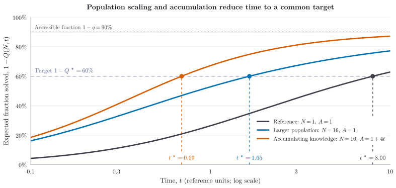
Figure 2 uses illustrative $a=0.5$, $b=1$, $q=0.1$, and $\lambda=0.57$. For $Q^\star=0.4$, Equation 2 gives $W^\star=8$. Constant-efficiency trajectories reach this target at $t^\star=8/N^{0.57}$; the learning trajectory $A(t,N)=1+4t$ reaches it when $N^{0.57}(t+2t^2)=8$. The plotted times are $8.00$, $1.65$, and $0.69$ in the chosen time units. Zero-success trials alone cannot distinguish a very low completion rate from structural inaccessibility.

A.3 Checkpoint completion work

Under restart, completion work is a hitting time for $m$ consecutive Bernoulli successes. With a checkpoint after every stage, completion work is $m$ plus a negative-binomial failure count. Figure 7 uses their exact 2.5th and 97.5th percentiles. Its $A$ is the ratio of expected work.

A.4 Value of continued evaluation

Under the Gaussian model in Section 3.5, the posterior variance after $n$ observations is $v_n=(\tau^{-2}+n\sigma^{-2})^{-1}$ and the posterior mean is $m_n=v_n(m/\tau^2+n\overline{Y}/\sigma^2)$. Before observing the data, $\overline{Y}\sim\mathcal{N}(m,\tau^2+\sigma^2/n)$, giving $\operatorname{Var}(m_n)=\tau^2-v_n=\tau^4/(\tau^2+\sigma^2/n)$. Integrating the positive part of a normal variable with mean $-\Delta$ and standard deviation $s_n$ gives $\mathbb{E}[(m_n-\mu_0)_+]=s_n\phi(\Delta/s_n)-\Delta\Phi(-\Delta/s_n)$.

Figure 10 plots this expression with $\Delta=\tau=1$, $\sigma=4$, $c=0.02$, and $M\in\{10,20,40\}$. With $g(n)=\mathbb{E}[(m_n-\mu_0)_+]$, an integer budget is profitable when $M>cn/g(n)$. The minimum of this threshold over positive integer budgets is approximately $12.73$, explaining why $M=10$ admits no profitable budget. Since $g(n)\leq g_\infty=\tau\phi(\Delta/\tau)-\Delta\Phi(-\Delta/\tau)$, any budget greater than $Mg_\infty/c$ has negative net value. Searching integer budgets up to this bound, together with the option $n=0$, therefore suffices to identify the best budget.

A.5 Efficiency evidence and workflow coverage

The estimates below measure improvements in original workloads and resource units. The coverage calculations are conditional scenarios for applying improvements of these magnitudes to a swarm’s workload.

For a local fourfold reduction in work, $A=1/(1-f+f/4)$ reaches two at $f=2/3$. A local factor of $4.9$ requires $f\simeq0.628$ for the same overall multiplier. For the inherited-learning factor of $9.58$, $$A=\frac{1}{(1-f)+f/9.58},\qquad A=5\ \Longleftrightarrow\ f\simeq0.893.$$ The $A=9.58$ scenario assumes that this improvement reaches the entire workflow. These calculations assume the measured local factor includes the recurring costs of applying the improvement, with acquisition costs assessed over subsequent use.

References

1. Toby Ord. Swarm Scaling. 2026.

2. OpenAI. GPT-5.6 model release. 2026.

3. Hidenori Tanaka. When Is Collective Intelligence a Lottery? Multi-Agent Scaling Laws for Memetic Drift in LLMs. 2026.

4. Guy E. Blelloch and Bruce M. Maggs. Parallel Algorithms. Chapter 25, Sections 25.2.2 and 25.2.4.

5. Richard S. Sutton. The Bitter Lesson. 2019.

6. Scaling Discovery through Test-Time Communication. Version 1. 2026.

7. Cynthia Dwork and colleagues. Generalization in Adaptive Data Analysis and Holdout Reuse. 2015.

8. Nina L. Corvelo Benz and colleagues. Evaluation of Large Language Models via Coupled Token Generation. AISTATS, 2026.

9. Rémy Degenne, Pierre Ménard, Xuedong Shang, and Michal Valko. Gamification of Pure Exploration for Linear Bandits. ICML, 2020.

10. AlphaEvolve. Version 1. 2025.

11. Discovering Multiagent Learning Algorithms with Large Language Models. Version 1. 2026.

12. Toby Ord. The Dynamics of Intelligence Explosions.

13. Raemon. Recursive Middle Manager Hell. 2023.

14. Noam Brown. Agent swarms, alignment, and recursive self-improvement. Interview with Dwarkesh Patel. 2026.

15. Anthropic. How we built our multi-agent research system. 2025.

16. Zaifeng Pan and colleagues. KVFlow: Efficient Prefix Caching for Accelerating LLM-Based Multi-Agent Workflows. Version 1. 2025.

17. Simon Schmitt and colleagues. Kickstarting Deep Reinforcement Learning. Version 1. 2018.

18. M. R. Garey, D. S. Johnson, and Ravi Sethi. The Complexity of Flowshop and Jobshop Scheduling. Mathematics of Operations Research, 1(2):117–129, 1976.

19. Sirui Hong and colleagues. MetaGPT: Meta Programming for A Multi-Agent Collaborative Framework. ICLR, 2024. Code repository.

20. Chen Qian and colleagues. Scaling Large Language Model-based Multi-Agent Collaboration. ICLR, 2025.

21. Wujiang Xu and colleagues. A-MEM: Agentic Memory for LLM Agents. NeurIPS, 2025.